A first computational notebook

Objectives

Get started with notebooks for analysis.
Get a feeling for the importance of execution order.

Instructor note

5 min teaching
20 min exercises

Creating a computational narrative

Let’s create our first real computational narrative in a Jupyter notebook (adapted from Python and R data analysis course at Aalto Science IT).

Picture of throwing darts — Throwing darts to compute pi.

Imagine you are on a desert island and wish to compute pi. You have a computer with you with Python installed but no math libraries and no Wikipedia.

Here is one way of doing it - “throwing darts” by generating random points within a square area and checking whether the points fall within the unit circle.

Launching JupyterLab notebook

In your terminal first create a folder or navigate to a folder where you would like the new notebook to appear.

After you have created a new folder and moved to it, launch JupyterLab:

$ jupyter-lab

This opens JupyterLab in your browser. Click on the Python 3 tile.

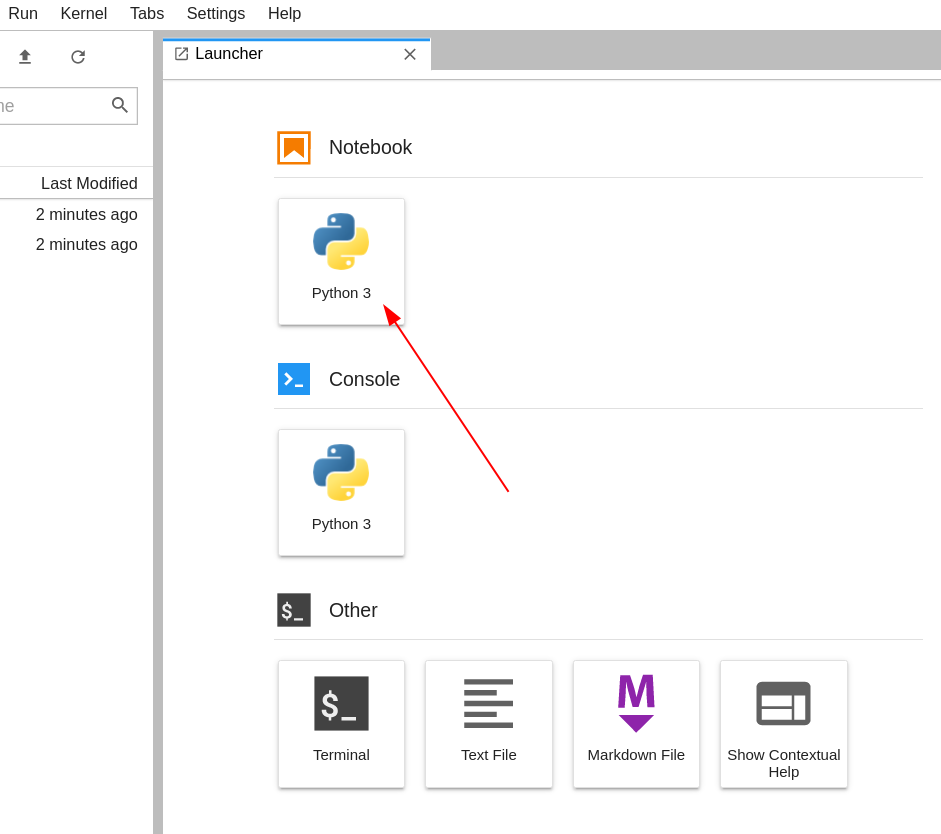
JupyterLab opened in the browser. Click on the Python 3 tile.

If you prefer to select in which browser to open JupyterLab, use:

$ jupyter-lab --no-browser

An example computational notebook

Hint: Opening a webpage inside JupyterLab

If you would like to copy-paste content from this webpage into your Jupyter notebook, a cool way of doing it is to open this page inside an IFrame:

from IPython.display import IFrame
IFrame(src="https://coderefinery.github.io/jupyter/first-notebook/", width='100%', height='500px')

Exercise/demonstration: Calculating pi using Monte Carlo methods

This can be either done as a 20 minute exercise or as a type-along demo.

Each numbered item will be a new cell. Press SHIFT+ENTER to run a cell and create a new cell below. With the cell selected, press ESCAPE to go into command mode. Use shortcuts M and Y to change cells to markdown and code, respectively.

Create a new notebook, name it, and add a heading (markdown cell).
```
# Calculating pi using Monte Carlo methods
```

Document the relevant formulas in a new cell (markdown cell):

## Relevant formulas

- square area: $s = (2 r)^2$
- circle area: $c = \pi r^2$
- $c/s = (\pi r^2) / (4 r^2) = \pi / 4$
- $\pi = 4 * c/s$

Add an image to explain the concept (markdown cell):

## Image to visualize the concept

![Darts](https://raw.githubusercontent.com/coderefinery/jupyter/main/example/darts.svg)

Import two modules that we will need (code cell):

# importing modules that we will need

import random
import matplotlib.pyplot as plt

Initialize the number of points (code cell):

# initializing the number of "throws"

num_points = 1000

“Throw darts” (code cell):

# here we "throw darts" and count the number of hits

points = []
hits = 0
for _ in range(num_points):
    x, y = random.random(), random.random()
    if x*x + y*y < 1.0:
        hits += 1
        points.append((x, y, "red"))
    else:
        points.append((x, y, "blue"))

Plot results (code cell):

# unzip points into 3 lists
x, y, colors = zip(*points)

# define figure dimensions
fig, ax = plt.subplots()
fig.set_size_inches(6.0, 6.0)

# plot results
ax.scatter(x, y, c=colors)

Compute the estimate for pi (code cell):

# compute and print the estimate

fraction = hits / num_points
4 * fraction

Here is the notebook: https://github.com/coderefinery/jupyter/blob/main/example/darts.ipynb (static version, later we will learn how to share notebooks which are dynamic and can be modified).

Instructor note

Demonstrate out-of-order execution problems and how to avoid them:

Add a cell at the end of the notebook which redefines num_points
Then run the cell which computes the pi estimate
Then demonstrate “run all cells”

Notebooks in other languages

It is possible to use Jupyter for other programming languages than Python (list of supported kernels). However, if you write R or Julia code, instead of installing a kernel, we recommend to use their corresponding notebook solutions which are optimized for these languages:

R Markdown for R
Pluto.jl for Julia

Discussion

What do we get from this?

With code separate from everything else, you might just send one number or a plot to your supervisor/collaborator for checking.
With a notebook as a narratives, you send everything in a consistent story.
A reader may still just read the introduction and conclusion, but they can easily see more - and try changes themselves - if they want.

Where should we add comments?

We can comment code either in Markdown cells or in the code cell as code comments.

What advantages do you see of commenting in Markdown cells and what advantages can you list for writing code comments in code cells?

Keypoints

Notebooks provide an intuitive way to perform interactive computational work.
Allows fast feedback in your test-code-refactor loop.
Cells can be executed in any order, beware of out-of-order execution bugs!